Tutorial : Introduction and Alanine Dipeptide¶

Move to tutorial directory, prepare trajectories¶

Assuming you’ve just downloaded and installed the package, move to the Tutorial directory.

$ cd Tutorial

Create an MSMBuilder Project¶

$ msmb ConvertDataToHDF  -s native.pdb -i XTC

Cluster your data¶

The following command clusters your data using the RMSD metric using a hybrid k-centers k-medoids approach. K-centers clustering continues until the intercluster distance (-d) is 0.045 nm. At that point, 50 iterations (-l) of hybrid k-medoids are performed to refine those clusters.

$ msmb Cluster rmsd hybrid -d 0.045 -l 50

After clustering, one must assign the data to the clusters. For the clustering settings used above, this happens automatically, so you will not need to run a separate assignment step. For other clustering protocols, you may need to run Assign.py or AssignHierarchical.py after the clustering phase.

The assignments of each conformation are stored as Data/Assignments.h5. The cluster centers are stored as Data/Gens.lh5.

Note that clustering with the RMSD metric requires a list of which atom indices to use during RMSD calculation. This file is typically called AtomIndices.dat and can typically be created using the script CreateAtomIndices.py. Because alanine dipeptide contains non-standard atom names, it cannot be generated automatically; a default AtomIndices.dat has already been placed in the Tutorial directory for your use. Note that AtomIndices.dat uses zero based indexing–the first atom in your system has index 0.

Alternative Clustering Protocols¶

Note that other clustering protocols (e.g. Ward’s algorithm) often leads to improved models; see the AdvancedMethods tutorial for details.

Validate microstate model with relaxation timescales.¶

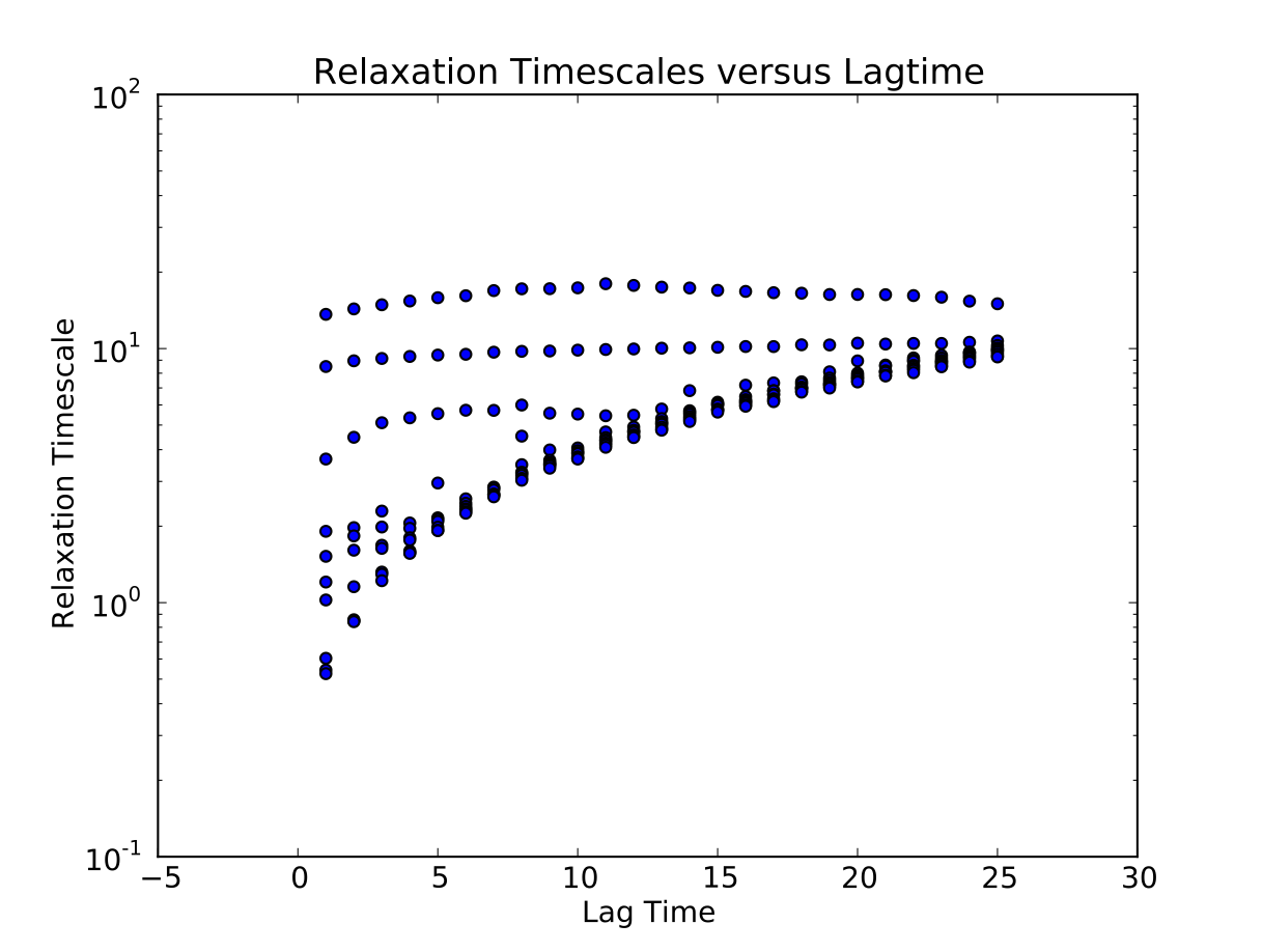
We calculate the relaxation timescales for a sequence of lagtimes \(\{1, 2, ..., 25\}\):

$ msmb CalculateImpliedTimescales -l 1,25 -i 1 -o Data/ImpliedTimescales.dat

Next, we use python to plot the results, specifying the lagtime between frames (1 ps):

$ msmb PlotImpliedTimescales -d 1. -i Data/ImpliedTimescales.dat

Construct MSM at appropriate lagtime¶

The plotted relaxation timescales suggest that the three slow timescales are reasonable flat at a lagtime of 3 timesteps [ps]. Thus, we construct an MSM using that lagtime:

$ msmb BuildMSM -l 3

At this point, MSMBuilder has written the following files into your ./Data/ directory:

Assignments.Fixed.h5
tCounts.mtx
tProb.mtx
Mapping.dat
Populations.dat

Assignments.Fixed.h5 contains a “fixed” version of your microstate assignments that has removed all data that is trimmed the maximal ergodic subgraph of your data.

tCounts.mtx contains the maximum likelihood estimated reversible count matrix. This is a symmetric matrix.

tProb.mtx contains the maximum likelihood estimated transition probability matrix.

Mapping.dat contains a mapping of the original microstate numbering to the “fixed” microstate numbering. This is necessary because some states may have been discarded during the ergodic trimming step.

Populations.dat contains the maximum likelihood estimated reversible equilibrium populations.

Construct a Macrostate MSM¶

Spectral clustering methods such as PCCA+ can be used to construct metastable models with a minimal number of states. You may also be interested in trying a Bayesian method called BACE that appears to outperform existing spectral methods. However, for the purpose of this Tutorial, we will focus on the more standard spectral methods.

First, we need to construct a microstate model with a short lagtime. The short lagtime is necessary because PCCA+ tries to create macrostates that are long-lived, or metastable. At long lagtimes, states become less and less metastable.

$ msmb BuildMSM -l 1 -o L1

Our previous examination of the relaxation timescales suggested that there were 3 slow processes, so we choose to build a model with 4 macroscopic states.

$ msmb PCCA -n 4 -a L1/Assignments.Fixed.h5 -t L1/tProb.mtx -o Macro4/ -A PCCA+

Examining the macrostate decomposition¶

It is known that the relevant degrees of freedom for alanine dipeptide are the phi and psi backbone angles. Thus, it is useful to examine (phi,psi). This data has been pre-calculated and is stored in Dihedrals.h5, or you can compute it via

$ python GetDihedrals.py --pdb native.pdb -a Macro4/MacroAssignments.h5 -n 1000

This will sample up to 1000 conformations from each macrostate. To sample all macrostates, use -n -1. We then visualize the data.

$ python PlotDihedrals.py Dihedrals.h5

You should see something like the following graph (our clustering and PCCA+ code both perform randomized searches, so your plot may appear slightly different):

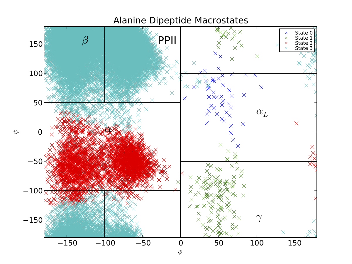
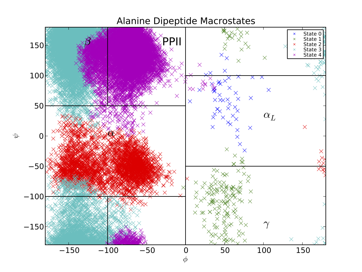
Thus, the PCCA algorithm has automatically identified the key basins of alanine dipeptide. The black lines correspond to the \(\beta, PP_{II}, \alpha_R, \alpha_L\) and \(\gamma\) conformational basins, as estimated previously . If we want a model that is less coarse grained, we can build a macrostate MSM with more states. If, for example, we had used 5 states, we would produce a Ramachandran plot that also captures the barrier between the \(\beta\) and \(PP_{II}\) basins.

In general, PCCA and PCCA+ are best applied to capturing long-lived, metastable states. Thus, for this system, applying PCCA+ to construct models with more than 5 states may not produce useful models. This is because alanine dipeptide only contains four eigenvalues that are significantly slower than the time resolution of 1 ps.

Calculate Macrostate Implied Timescales¶

$ msmb CalculateImpliedTimescales -l 1,25 -i 1 \
-o Macro4/ImpliedTimescales.dat -a Macro4/MacroAssignments.h5 -e 3

$ msmb PlotImpliedTimescales -i Macro4/ImpliedTimescales.dat -d 1

Occasionally, PCCA+ will lead to poor macrostates, so it is important to verify that:

1. The state decomposition makes physical sense
2. The macrostate implied timescales make sense
3. The macrostate implied timescales “follow” the microstate implied timescales

Furthermore, PCCA+ is best used to estimate metastable states. Here are some additional guidelines for achieving good success with PCCA+:

1. If your microstate model has too long of a lagtime, the model may not be metastable because significant dynamics occurs on the timescale of a single lagtime.
2. If your microstate model has too short of a lagtime, the microstate model may not be Markovian, leading to errors when estimating the eigenvalues and eigenvectors. Most importantly, significant non-Markovian dynamics can cause the slowest eigenvalues to be mis-identified. If this occurs, your PCCA+ model will be worthless! To prevent this, a useful guide is to make sure that the slowest implied timescales do not cross one another (e.g. their rank ordering is constant).
3. If your microstate model has too few states, your microstate model may not be sufficiently Markovian. You may not have sufficient geometric resolution to accurately identify the primary kinetic barriers.
4. If your microstate model has too many states, your microstate model will have poor statistics, possibly leading to poor estimates of the slow eigenvectors.

Thus, success with PCCA+ may require some trial and error when selecting the appropriate lagtime and microstate clustering. Finally, note that our implementation of PCCA+ uses a simulated annealing minimization. This randomized search means that you may find multiple minima by repeating the PCCA+ calculation several times. You may find a better model by repeating the calculation several times.

Visualizing Structures with Pymol¶

Because macrostate models typically have a handful of states, it is easy for humans to compare the resulting structures visually. One way to do this is to save randomly selected conformations from each state, then view them in Pymol (or VMD):

$ msmb SaveStructures -s -1 -f pdb -S sep -a Macro4/MacroAssignments.h5
pymol PDBs/State0-0.pdb PDBs/State1-0.pdb PDBs/State2-0.pdb PDBs/State3-0.pdb

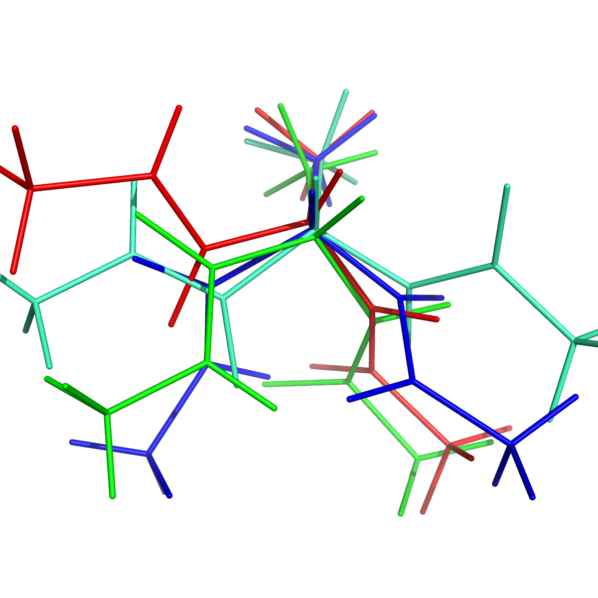
Randomly selected conformations from the four macrostate model. Colored by macrostate.