Time-Structure Based Independent Component Analysis (tICA)¶

Introduction¶

The time-structure based Independent Component Analysis (tICA) method as applied to MSM construction is a new way to judge distances in the protein conformational landscape. The strategy will be to define a reduced dimensional representation of the protein conformations, and use distances in this space in the clustering step of the MSM construction process. Consider a single, long trajectory from a simulation, \(\mathbf{X}(t) \in \mathbb{R}^d\), which has \(d\) dimensions each corresponding to some structural degree of freedom (such as a single phi angle).

One natural way we could define the reduced space is to use Principal Component Analysis, or PCA (See Gerhard Stock’s work for examples). In PCA, the goal is to find projection vectors that maximize their explained variance, subject to them being uncorrelated and having length one. In the end, these maximal variance projections correspond to the solutions of the following eigenvalue problem:

\[\Sigma v = \lambda v\]

where \(\Sigma\) is the covariance matrix given by:

\[\Sigma_{ij} = \mathbb{E}\Big[ X_i(t) X_j(t) \Big]\]

The problem with using PCA to define the reduced space, however, is that high-variance degrees of freedom need not be slow (for instance consider a floppy protein tail that varies wildly vs. a single dihedral angle that is required to rotate for a protein to fold). What we really want is to design projections that can best differentiate between slowly equilibrating populations, which is precisely where tICA comes in.

In tICA, the goal is to find projection vectors that maximize their autocorrelation function, subject to them being uncorrelated and having unit variance. It is easy to show (see Schwantes, CR and Pande, VS. JCTC 2013, 2000-2009.) that the solution to the tICA problem are the solutions to this generalized eigenvalue problem (which is closely related to the PCA eigenvalue problem):

\[C^{(\Delta t)} v = \lambda \Sigma v\]

where \(C^{(\Delta t)}\) is the time lag correlation matrix defined by:

\[C^{(\Delta t)}_{ij} = \mathbb{E}\Big[ X_i(t) X_j(t+\Delta t) \Big]\]

Given this solution, we can use the tICA method to define a reduced dimensionality representation of each \(\mathbf{X}(t)\) by projecting the vector onto the slowest \(n\) tICs. Therefore, the strategy for using tICA to construct an MSM looks like:

Calculate \(C^{(\Delta t)}\) and \(\Sigma\) and the solutions to the generalized eigenvalue problem given above
Choose the number of tICs to project onto
Use the reduced space to cluster and assign conformations to states
Build the MSM from these assignments and analyze as laid out in the MSMBuilder tutorial

In the next section we will go over how to do each of these steps within MSMBuilder.

Selection of tICA Parameters¶

There are two parameters introduced in the tICA method. The first is \(\Delta t\), which is used in the calculation of the time-lag correlation matrix (\(C^{(\Delta t)}\)). The second is \(n\), which is the number of tICs to project onto when calculating distances between conformations.

There is currently no optimal method for choosing these parameters, however, the method has been fairly robust to different choices.

In previous analyses of Fip35, villin, NTL9(1-39), and NuG2, \(\Delta t\) between 50 and 1000 nanoseconds produced MSMs with largely the same timescale distribution, indicating that something in this range should be appropriate for most protein systems.

MSMs are more sensitive, however, to the selection of the number of tICs to project onto. In the previous analyses listed above, we found that using a surprisingly small number (in the range of 5-20) of tICs worked well. The power behind tICA is to ignore the degrees of freedom that quickly decorrelate and only add noise in the distance calculation. However, as \(n\) gets smaller (and we throw out more degrees of freedom), the resolution of the MSM becomes limited, and can only discern between conformations along the slowest coordinate (which is often the folding process).

For example, in our analysis of NTL9, we found that increasing \(n\) from three up to seven kept the folding timescale largely unchanged but added new microsecond timescales to the resulting MSMs, while adding in too many (\(> 10\)) produced a folding timescale that was too fast.

Understanding the tICs¶

The top tICs represent linear combinations of the input degrees of freedom that decorrelate slowly. These vectors are not necessarily easy to visualize, however.

For instance, the slowest tIC from the above analysis can be visualized as a matrix, where each entry corresponds to the tIC entry corresponding to a pair of atoms’ distances.

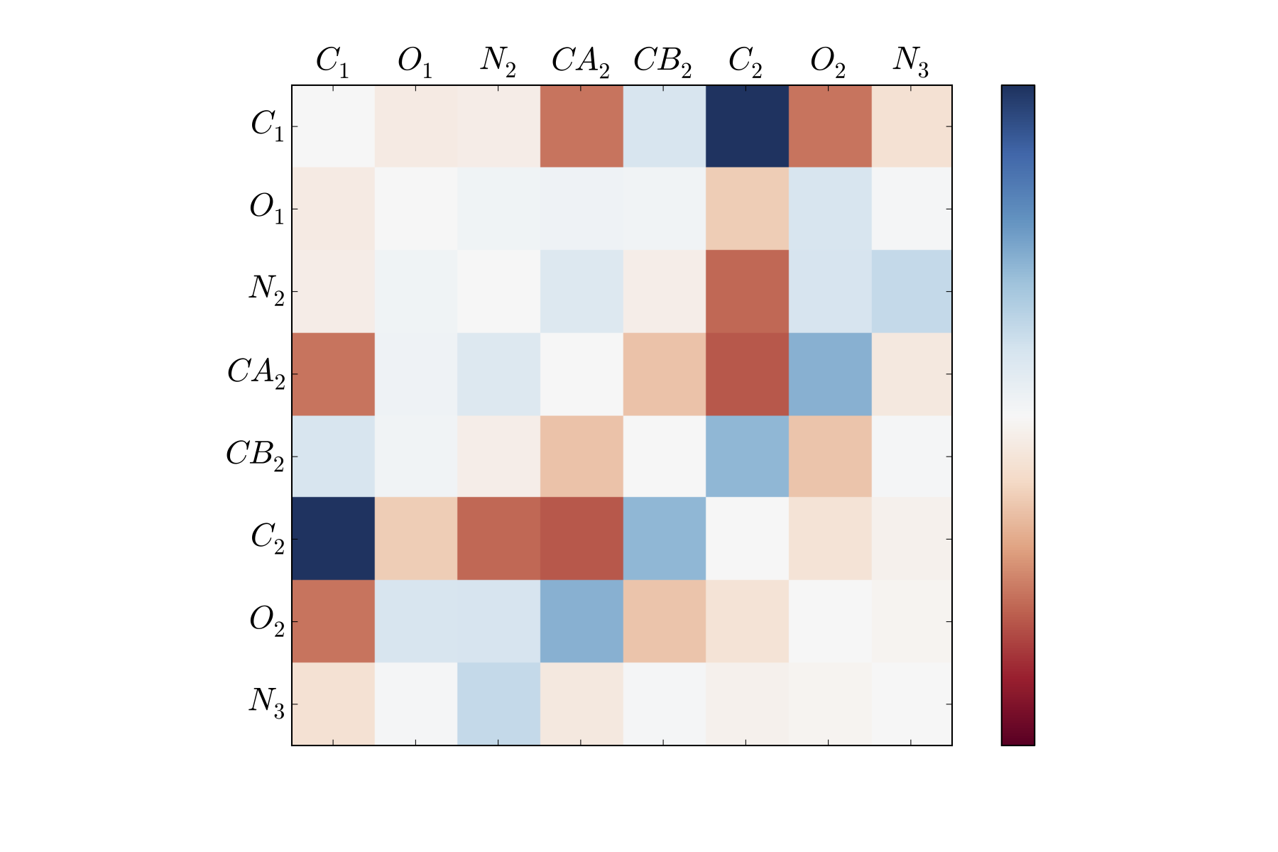
Here, the dark blue and dark red portions correspond to atom pairs that best distinguish between far regions along the first tIC. As is clear, this is not all that helpful to look at (though an area that could be greatly improved is providing a visualization tool for these degrees of freedom).

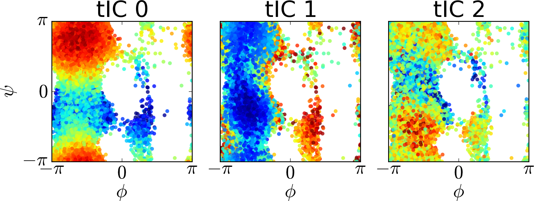
We can also attempt to visualize the tICs by comparing the projections onto each tIC to order parameters. For instance, for each conformation we sampled in the reference simulations, we can calculate the phi and psi angles along with the projection of the conformation onto each tIC. In this way, we can visualize what each tIC corresponds to. Below, we have plotted the phi and psi angles colored by that conformation’s projection onto each tIC.

Drawbacks of tICA¶

Since part of the process of using tICA is a dimensionality reduction, there is always the opportunity to throw out important pieces of information. In particular, by throwing out the faster degrees of freedom, we can better estimate the slowest timescales; but this comes with the trade-off of not representing the fast timescales correctly. The result is illustrated when trying to sample a trajectory from the MSM built on tICA. The result is a trajectory that represents the folding/unfolding transition well, but when in the unfolded state jumps around more than would be seen in a typical MD simulation.